How to Create a Day Series in Excel Column

Create a Day Series in Excel Column

Hi..

      Readers ! Let us learn how to Create a day series in 'Date' in Excel sheet, Here We make continuously changing 'Day' in the 'date' format in a column series while drag mouse pointer. Even we can make to changing 'Month' or 'Year' continuously by using this tip.   follow the below steps to make this easy.

Step 1:

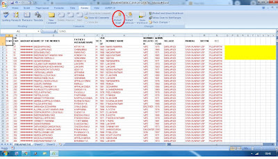
in the above picture

1. first enter a date '01-20-2001' in column 'A' in cell 'A1'

2. select entire column 'A'

3. Home tab -> fill -> Click 'series' 

4. now pop-up will come like above screen

5. enable series in 'Column'

6. enable Type 'Date'

7. enable Date unit 'Day'

8. Click to 'Ok' 

Now you will changing day in date series in column 'A' , Now you can try for Month, Weekday or Year same like this. 

Thank you

Excel tric blog

Fill Number Series in Excel Column

How to Fill Number Series in Excel Column

Hi.!
     In this Tutorial We are providing how to fill number series in excel column with using mouse and drag them. Ya this is most useful because if we want more than 1000 numbers in series in a single column it is very difficult to drag them with your mouse even it takes more time. So learning this we can make how to number series an easy way below steps to guide you how to do this process.

step 1:

1. enter number 1 & 2 in column 'A'.
2. Now select entire column 'A'
3. Home Tab -> Fill -> Click 'series' Option

4. now you will see a pop-up window, make sure enable 'Column' radio button
5. enable Type 'Linear' 
6. Set Step value to '1'
7. Set stop value to '1000'
8. Click to 'Ok' Button 
Now you will see 1000 numbers in Sequential Order in Column 'A'.


Thank You
Excel Tric blog 

How to use 'MERGECELLS' in Excel sheet

Hi. Readers!

in this lesson we are going to learn how to use 'MERGECELLS' in excel, this feature is very important feature in excel sheet, many people use mergecells for merge multiple cells as a single cell and add their text into center position of the cells like report titles, project heading ect. Let us see how do the mergecells in excel sheet, watch below steps how to create mergecells.

using merge cells in excel

steps:
1. select more than two cells in your excel sheet row or column
2. Go to Home Tab -> click 'MERGECELLS' -> Click 'merge & center' option.
3. now, enter your text into this cell.
4. then press enter , your text position will be exact center of the cell.

How to use 'WRAPTEXT' in Excel sheet

Hi.Readers !

Welcome to exceltric.blogspot.in ! in this lesson we are going to explain you about using 'Wraptext' option in excel sheet. normally 'wraptext' option is most useful feature in excel sheet, using this we can adjust multi line text in one cell without overlap to next cell. Mostly data entry operators use this feature widely.
       If you want to enter Customer address or any product description in one cell in excel sheet this will be used as per given example below. Just watch below steps to learn how to use 'wraptext' feature in excel.

Example :

How to use textwrap in excel

Steps :
1.  Select any one cell in excel sheet
2. go to Home Tab -> Click on 'wraptext'
3. Now keep typing you text (ex; address )
Note: don't press enter button till finish typing complete address.
4. Now, Press Enter -> Adjust cell height and width with mouse as per given about.
5. you can use text alignments to adjust your text into exact center position of the cell.

How to use Pivot Tables in Excel

What is a Pivot Table ?

Pivot tables helps to Classify and Summarising complicated  data into a simple easy drill down in details.

Step1 :

in the above given table, Different product sold in different Quarters So we can find easily classify and summarise the above content using Pivot tables.

Step 2:












Select entire table and Click insert menu -> Pivot tables -> Pivot tables option.



Step3:

enable 'new worksheet' -> click to 'Ok'



Step4:
now, new work sheet will be added beside your sheet, there you find a pivot table design block and pivot table elements panel in the right side of window as show below.

step5:
now, drag 'Products'  and drop into 'row labels , Similarly drag 'sale' and drop into 'Sum values' , similarly drag 'Quarter' and drop into 'report filters' as show below.

Now , see your pivot table Arrangement, now you can filter data in any manner.


thank you
excel tips

How to use SORT in Excel

Hi..Readers !

In this lesson you can learn how to Arrange Records in A-Z or Z-A Order we also called SORT Order in Excel sheet. Watch below Steps


Steps 1:


Create a Table as per given below

 A                    B                    C
Slno               name             Salary
105                    Anthony          15000
108                    David              17000
103                    Misra                25000
104                   Vasavi              28000




Step2:
Select above table ->  Go to 'DATA' Menu  -> Click 'SORT'


 Step3:
 Now select 'Ascending (A-Z) Order ->  Click 'Ok'


Now Your Table will be like this



Slno               name             Salary
103                    Misra                25000
104                   Vasavi              28000
105                    Anthony          15000
108                    David              17000

How to Hide or Show Worksheets in Excel

Show or Hide Worksheets 

It is very easy. You can hide any sheet in your excel work book. when ever you want you can make sheet visible. follow the below steps to make hide sheets or show sheets in excel workbook

step 1:

in the above screen shot, We have 3 sheets by default in excel workbook, to Hide sheet 1 , right click on sheet click to 'Hide' option.

Step 2:

Once you click hide button, you are able to see only 2 sheets in your workbook,

Steps for Unhide Sheet

1.right click and Click 'Unhide' 
2.Select Your Sheet 1
3.Click to 'OK'